Vision Transformer (ViT), specifically designed for the Computer Vision (CV) field, is an AI architecture that utilizes the Transformer architecture to process visual data.

This post will follow through the paper "An Image is Worth 16x16 Words: Transformers for Image Recognition at Scale" by Dosovitskiy et al. [1], introducing the concept of the Vision Transformer model and evaluating its performance in CV tasks in detail. An example code of the model is also included.
Table of Contents:
1. Background
1-1. What Are Transformers and Self-Attention?
1-2. What is CNN and Why is it So Popular in the Computer Vision Field?
1-3. Attempts to Utilize Transformers in the Computer Vision Field
2. Vision Transformer (ViT)
2-1. Model Overview
2-2. Model Design Details
2-3. Code Implementation
2-4. Additional Information
3. Experiment and Performance Analysis
3-1. Setup
3-2. Comparison to the State of the Art
3-3. Limitations
4. Conclusion
5. References
1. Background
1-1. What Are Transformers and Self-Attention?
The Transformer is a neural network architecture based on the multi-head attention mechanism, first introduced in the 2017 paper "Attention Is All You Need," by Vaswani et al [2]. This architecture transforms texts into number codes known as "tokens" and then analyzes the tokens to understand the context. During this process, important words are amplified, while less important words are diminished. The architecture mainly consists of two parts: encoder and decoder. Both encoder and decoder utilize stacked self-attention and point-wise, fully connected layers. The encoder is used to process input data and the decoder is used to generate output sequences (e.g. translation of the input text) [2].

The biggest advantage of transformers is that they don't have to perform multiple calculations like other AI models. This makes the model faster to train and allows the model to understand much longer texts. ChatGPT is a famous example of a transformer-based model [3].
Transformers specifically utilize a mechanism called "self-attention" to understand longer texts. Self-attention considers other elements in the sequence, including itself, and understands the context through analyzing the relationship between those elements. Ultimately, self-attention allows transformers to capture dependencies between elements far apart, allowing the model to understand the text as a whole [4]. The detailed implementation of the attention mechanism is thoroughly explained in the original paper ("Attention is All You Need").
1-2. What is CNN and Why is it So Popular in the Computer Vision Field?
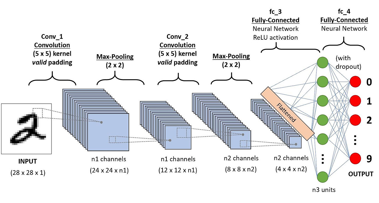
CNN is a deep learning model consisted of three main layers: convolutional layer, pooling layer, and fully connected layer. In the convolutional layer, CNNs extract important features using small filters (kernels). In the pooling layer, only the most important features are kept, while other areas are disregarded, minimizing the computation cost. The fully connected layers connect all the layers and make a final prediction based on the extracted features.
The powerful, yet efficient nature of CNN allowed it to become the most widely used model in the CV field, also allowing the model based on CNN to achieve state-of-the-art (SOTA) performance [5].
1-3. Attempts to Utilize Transformers in the Computer Vision Field
There have been many attempts to incorporate transformers in the traditionally CNN-dominated CV field, mainly because of its outstanding performance in NLP. Unlike in NLP, applying the self-attention mechanism to all the pixels in an image was unrealistic as it was too computation-heavy. Researchers have employed different techniques to utilize the strengths and avoid the limitations of transformers.
1. Local Self-Attention:
Parmar et al. applied self-attention to only local neighborhoods for each query pixel [6].
2. Sparse Transformers:
Child et al. employed scalable approximations to global self-attention in order to reduce the computation cost and make it applicable to images [7].
3. Blocks of Varying Sizes:
Weissenborn et al. applied self-attention in blocks of varying sizes or even only along individual axes to increase efficiency [8].
4. Combining CNN and Self-Attention
Many researchers experimented with combining CNNs and self-attention by augmenting feature maps or further processing the output of CNN using self-attention.
2. Vision Transformer (ViT)
2-1. Model Overview
Unlike other attempts, ViT strictly follows the original Transformer design to utilize the scalable NLP Transformer architectures, and their efficient implementations, right away without any special modifications. ViT divides the image into small patches (instead of traditional CNN filters), and processes them one by one like text tokens in NLP.
Simply put, instead of designing a specialized layer for image processing, ViT makes an image act like a block of text with words (small patches). This approach allows the Transformer architecture used in NLP to be directly applied in CV tasks without any modifications.
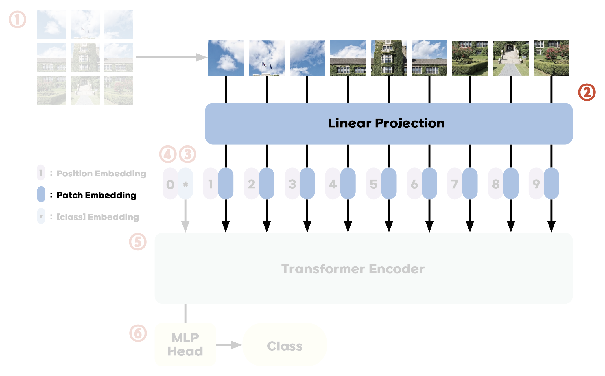
A brief overview of the model:

1. Divide an image into small patches, called tokens, with equal size.
2. Flatten the patches into vectors and embed them linearly.
3. Add positional embeddings to preserve spatial information.
4. Add a learnable classification token to the sequence.
5. Feed the sequence of tokens into the classical Transformer encoder.
6. Attach classification head to the [class] token throughout the training process to help with classification task.
2-2. Model Design Details
Step 1. Divide the Image into Small Patches

Divide the input image into small P X P sized patches, or what is known as tokens in NLP. The number of patches will be $N = HW / P^{2}$ where $(H, W)$ is the resolution of the original image. The number of patches is also equivalent to the length of the input sequence for the Transformer.
Step 2. Create Patch Embeddings
Flatten the patches into vectors and map to D dimensions with a trainable linear projection, as Transformers require constant latent vector size D for all of its layers. The output is called the patch embeddings.
Step 3. Add [class] Token
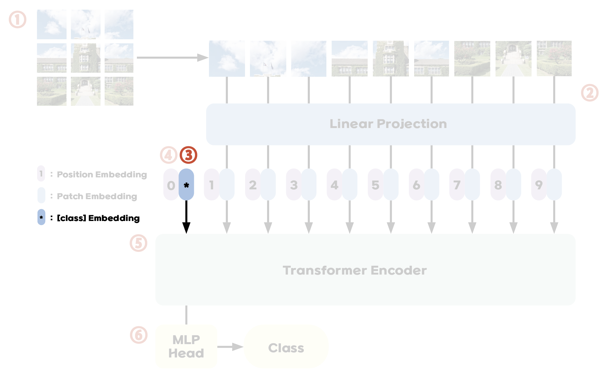
Like the BERT model's [class] token, a special learnable embedding is added at the front of the created patch embeddings. This token allows the model to summarize key characteristics of the image during the training process. After passing through multiple layers of the Transformer encoder, the token begins to gradually capture the general information of the image. After passing through the Transformer encoder and applying layernorm, this token output finally becomes the image representation $\mathbf{y}$ of the original image ($\mathbf{y} = \text{LN}(\mathbf{z}^{0}_{L})$)
Step 4. Add Position Embeddings
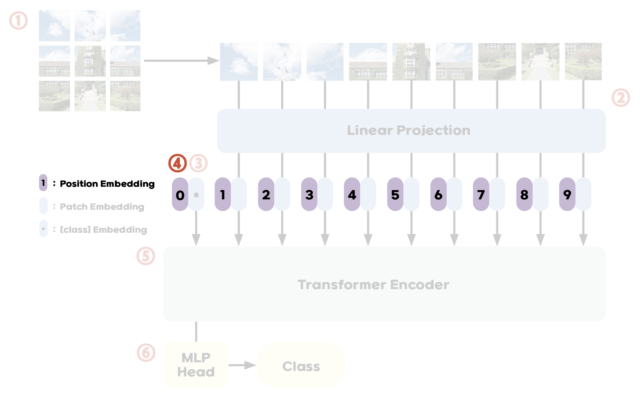
To maintain positional information, position embeddings are added to the patch embeddings. Although there are more complex 2D-aware position embeddings, standard learnable 1D position embeddings are used as 2D-aware ones lack significant performance gains. The final output sequence is then fed into the Transformer encoder.
Creating a sequence of embedding vectors $\mathbf{z}_0$ to be fed into the Transformer encoder can be explained simply by using the following equation, introduced in the paper:
$$\mathbf{z}_0 = \left[ \mathbf{x}_{\text{class}} ; \mathbf{x}_p^1 \mathbf{E} ; \mathbf{x}_p^2 \mathbf{E} ; \cdots ; \mathbf{x}_p^N \mathbf{E} \right] + \mathbf{E}_{\mathit{pos}}, \quad \mathbf{E} \in \mathbb{R}^{(P^2 \cdot C) \times D}, \quad \mathbf{E}_{\mathit{pos}} \in \mathbb{R}^{(N+1) \times D}$$
The input sequence is created by combining [class] token $\mathbf{x}_{\text{class}}$, patch embeddings $\mathbf{x}_p^1 \mathbf{E} ; \mathbf{x}_p^2 \mathbf{E} ; \cdots ; \mathbf{x}_p^N \mathbf{E}$, and position embedding $\mathbf{E}_{\mathit{pos}}$.
Step 5. Passing Through the Transformer Encoder

The processed input is fed into The Transformer encoder. The Transformer encoder consists of multiple layers of encoder blocks. Each encoder block consists of alternating multihead self-attention (MSA) and multi-layer perceptron (MLP) blocks. Before each block, layernorm is applied for training stabilization and it is residually connected to the output side of each block.
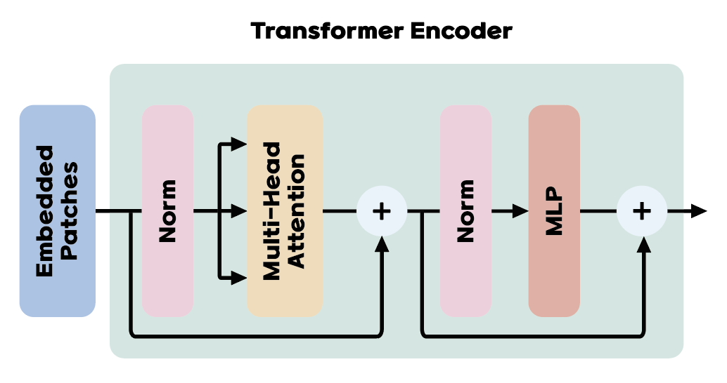
The Transformer encoder can also be explained using the equations:
$$\mathbf{z}'_{\ell} = \text{MSA}(\text{LN}(\mathbf{z}_{\ell-1})) + \mathbf{z}_{\ell-1}, \quad \ell = 1 \dots L
\\
\mathbf{z}_{\ell} = \text{MLP}(\text{LN}(\mathbf{z}'_{\ell})) + \mathbf{z}'_{\ell}, \quad \ell = 1 \dots L$$
The first equation is the first block of the Transformer encoder's MSA block. The ouput from $\ell-1$ layer ($\mathbf{z}_{\ell-1}$) is normalized and feed into MSA block $\text{MSA}(\text{LN}(\mathbf{z}_{\ell-1}))$. Then the output from the previous layer is connected to the output from the MSA block (residual connection). The same thing happens with the MLP block, but it additionally contains two layers with a GELU non-linearity.
Step 6. Output and Classification

The classification head is attached to [class] token $\mathbf{z}^{0}_{L}$ during pre-training and fine-tuning. This classification head helps the model to classify the image into the correct category. It is made of MLP with one hidden layer for pre-training and a single linear layer for fine-tuning.
2-3. Code Implementation
To see the example code implementation of the model provided by the authors of the paper, click below [9]:
import torch
from torch import nn

from einops import rearrange
from einops.layers.torch import Rearrange

# helpers

def pair(t):
    return t if isinstance(t, tuple) else (t, t)

def posemb_sincos_2d(h, w, dim, temperature: int = 10000, dtype = torch.float32):
    y, x = torch.meshgrid(torch.arange(h), torch.arange(w), indexing="ij")
    assert (dim % 4) == 0, "feature dimension must be multiple of 4 for sincos emb"
    omega = torch.arange(dim // 4) / (dim // 4 - 1)
    omega = 1.0 / (temperature ** omega)

    y = y.flatten()[:, None] * omega[None, :]
    x = x.flatten()[:, None] * omega[None, :]
    pe = torch.cat((x.sin(), x.cos(), y.sin(), y.cos()), dim=1)
    return pe.type(dtype)

# classes

class FeedForward(nn.Module):
    def __init__(self, dim, hidden_dim):
        super().__init__()
        self.net = nn.Sequential(
            nn.LayerNorm(dim),
            nn.Linear(dim, hidden_dim),
            nn.GELU(),
            nn.Linear(hidden_dim, dim),
        )
    def forward(self, x):
        return self.net(x)

class Attention(nn.Module):
    def __init__(self, dim, heads = 8, dim_head = 64):
        super().__init__()
        inner_dim = dim_head *  heads
        self.heads = heads
        self.scale = dim_head ** -0.5
        self.norm = nn.LayerNorm(dim)

        self.attend = nn.Softmax(dim = -1)

        self.to_qkv = nn.Linear(dim, inner_dim * 3, bias = False)
        self.to_out = nn.Linear(inner_dim, dim, bias = False)

    def forward(self, x):
        x = self.norm(x)

        qkv = self.to_qkv(x).chunk(3, dim = -1)
        q, k, v = map(lambda t: rearrange(t, 'b n (h d) -> b h n d', h = self.heads), qkv)

        dots = torch.matmul(q, k.transpose(-1, -2)) * self.scale

        attn = self.attend(dots)

        out = torch.matmul(attn, v)
        out = rearrange(out, 'b h n d -> b n (h d)')
        return self.to_out(out)

class Transformer(nn.Module):
    def __init__(self, dim, depth, heads, dim_head, mlp_dim):
        super().__init__()
        self.norm = nn.LayerNorm(dim)
        self.layers = nn.ModuleList([])
        for _ in range(depth):
            self.layers.append(nn.ModuleList([
                Attention(dim, heads = heads, dim_head = dim_head),
                FeedForward(dim, mlp_dim)
            ]))
    def forward(self, x):
        for attn, ff in self.layers:
            x = attn(x) + x
            x = ff(x) + x
        return self.norm(x)

class SimpleViT(nn.Module):
    def __init__(self, *, image_size, patch_size, num_classes, dim, depth, heads, mlp_dim, channels = 3, dim_head = 64):
        super().__init__()
        image_height, image_width = pair(image_size)
        patch_height, patch_width = pair(patch_size)

        assert image_height % patch_height == 0 and image_width % patch_width == 0, 'Image dimensions must be divisible by the patch size.'

        patch_dim = channels * patch_height * patch_width

        self.to_patch_embedding = nn.Sequential(
            Rearrange("b c (h p1) (w p2) -> b (h w) (p1 p2 c)", p1 = patch_height, p2 = patch_width),
            nn.LayerNorm(patch_dim),
            nn.Linear(patch_dim, dim),
            nn.LayerNorm(dim),
        )

        self.pos_embedding = posemb_sincos_2d(
            h = image_height // patch_height,
            w = image_width // patch_width,
            dim = dim,
        )

        self.transformer = Transformer(dim, depth, heads, dim_head, mlp_dim)

        self.pool = "mean"
        self.to_latent = nn.Identity()

        self.linear_head = nn.Linear(dim, num_classes)

    def forward(self, img):
        device = img.device

        x = self.to_patch_embedding(img)
        x += self.pos_embedding.to(device, dtype=x.dtype)

        x = self.transformer(x)
        x = x.mean(dim = 1)

        x = self.to_latent(x)
        return self.linear_head(x)
2-4. Additional Information
Inductive Bias
ViT has a comparably lower inductive bias on images than CNNs. CNN considers the 2D neighborhood structure of an image and its inability to move throughout all layers. In ViT, only the MLP layers act CNNs while self-attention layers are global. Therefore, ViT has to learn the spatial information and relational information of patches from scratch.
Hybrid Architecture
ViT can also utilize feature maps from CNNs as input instead of image patches. In this hybrid model, patch embedding projection $\mathbf{E}$ is applied to patches attained from CNN feature maps to convert them into a form suitable for ViT. Patches with 1x1 spatial size are also obtainable by flattening the spatial dimension of the feature map. The embeddings required for the Transformer are applied accordingly as explained above.
Fine-Tuning and Higher Resolution
ViT is pre-trained with a large dataset and later fine-tuned to smaller tasks. To do this pre-trained prediction head is replaced with a feed-forward layer with an initial value of 0. The amount of feed-forward layer is equivalent to the number of smaller tasks. If the resolution of an image increases, the effective sequence length increases as the patch size remains the same. In this case, the pre-trained position embeddings might become useless. To resolve this problem, 2D interpolation of the pre-trained position embeddings is performed.
3. Experiment and Performance Analysis
3-1. Setup
Dataset
ViT was trained with large datasets, such as ImageNet-21k which has 14M images and 21K classes, or JFT which has 303M high-resolution images and 18K classes. Experiments have proven that ViT pre-trained in a large dataset, especially the JFT-300M dataset, performs extremely well. This result is because ViT lacks inductive bias compared to CNNs. Since ViT has to learn the spatial information and relational information of patches from scratch, it requires large data to make the model learn the image structure efficiently. Pre-training ViT with large datasets and then fine-tuning to smaller benchmark datasets, such as, ImageNet and CIFAR-100 showed high performance, even comparable to SOTA CNNs.

Model Variants
ViT models are divided into three categories, based on the size of the model: Base, Large, and Huge. ViT-Base and ViT-Large models are configured based on BERT, while ViT-Huge is a newly created model. ViT models are denoted based on the model size and patch size. For example, ViT model that is large with a patch size of 16x16 is denoted ViT-L/16.

The Base CNN model used in the experiment is ResNet, but with Group Normalization, instead of Batch Normalization. Standardized convolutions are also used to improve transfer learning. For the hybrid models, feature maps from CNNs are fed into ViT with a patch size of one pixel.
Training and Fine-Tuning
For training every model, Adam optimizer with $\beta_1 = 0.9$, $\beta_2 = 0.999$ was used. Batch size and weight decay were set to 4096 and 0.1 respectively. Although SGD is more frequently used in ResNet training, Adam performed better in this study. Linear learning rate warmup and decay method was utilized. In the fine-tuning step, SGD with momentum was used with a batch size of 512. For the ImageNet dataset, ViT-L/16 model was fine-tuned to 512 resolution and 518 for ViT-H/14. Polyak & Juditsky averaging with a factor of 0.9999 was used to increase the model stability.
3-2. Comparison to State of the Art
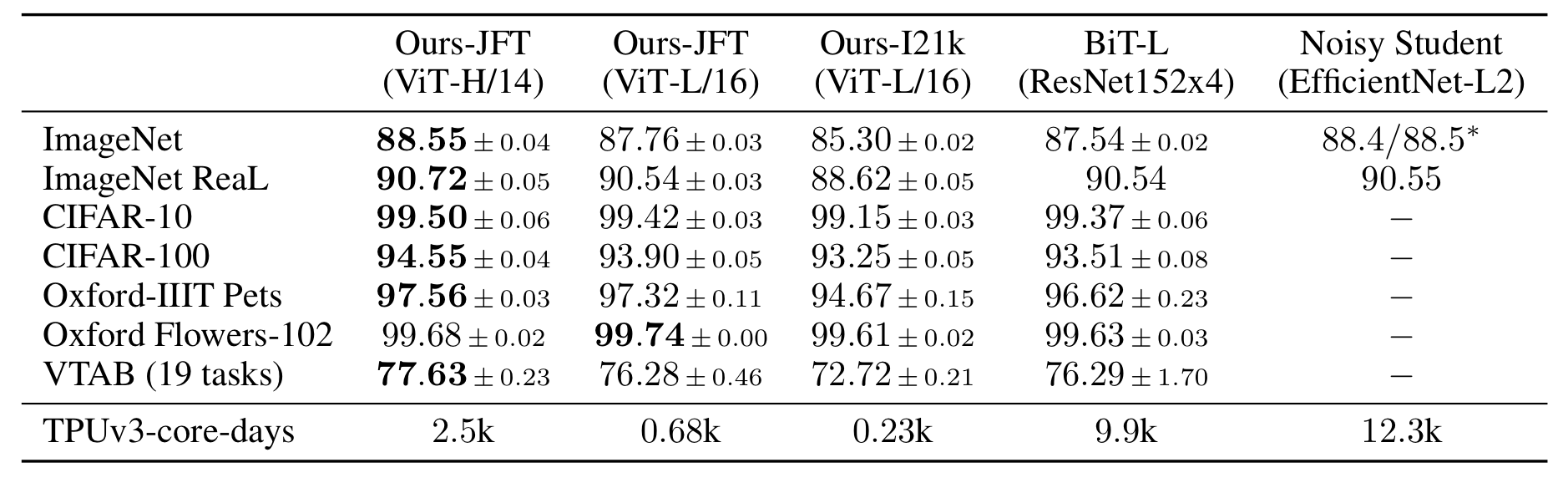
As can be seen in Table 2, the ViT model pre-trained with JFT-300M had higher accuracy than ResNet in every benchmark. Even comparably smaller ViT-L/16 already outperformed ResNet. The larger ViT model ViT-H/14 showed even higher performance in all the benchmarks, especially in more difficult benchmarks like ImageNet, CIFAR-100, and VTAB. The computational resources required for training ViT models were also much lower compared to those of ResNet and Noisy Student.
Although ViT-L/16 pre-trained on a slightly smaller dataset ImageNet-21K shows less accuracy than that of ResNet, it still shows fairly high performance considering the extremely low computational resources to train. Using this dataset, it only requires 30 days to train with 8-core TPUv3.

Also, hybrid models showed promising results in smaller models but became less significant as the model size grew. In summary, ViT models show better performance with fewer computational resources compared to CNN models. ViT models show high performance especially when pre-trained in large datasets.
3-3. Limitations
Unlike the BERT in NLP, the self-supervised learning method underperforms compared to supervised learning in ViT. Since self-supervised learning is one of the reasons why Transformers became so popular in NLP, successfully applying self-supervised learning to ViT will be extremely beneficial. Also, although ViT shows outstanding performance in classification tasks, more tuning is required to apply ViT to other CV tasks like object detection and segmentation.
4. Conclusion
This research directly contributed to a new method of applying the Transformer model directly to image classification tasks. Unlike other research that added inductive biases into the architecture, this research divided an image into small patches and trained sequentially like the Transformer model in NLP. This methodology is extremely simple, yet very powerful when pre-trained in a large dataset. Consequently, ViT performs on par with other SOTA CNN models in classification tasks with relatively low training costs.
As the ViT-based model (OmniVec) now holds state-of-the-art performance in image classification tasks (as of October 2024), understanding the archictecture and underlying concepts of ViT will be beneficial for those interested in the field of Computer Vision. The continued integration of different models and ideas will allow the relatively stagnant CV field to advance once more, as CNN architectures did.
5. References
[1] Alexey Dosovitskiy, Lucas Beyer, Alexander Kolesnikov, Dirk Weissenborn, Xiaohua Zhai, Thomas Unterthiner, Mostafa Dehghani, Matthias Minderer, Georg Heigold, Sylvain Gelly, Jakob Uszkoreit, and Neil Houlsby. An image is worth 16x16 words: Transformers for image recognition at scale. In ICLR, 2021.
[2] Ashish Vaswani, Noam Shazeer, Niki Parmar, Jakob Uszkoreit, Llion Jones, Aidan N. Gomez, Lukasz Kaiser, and Illia Polosukhin. Attention is All You Need. In NIPS, 2017.
[3] Amazon Web Services. What are Transformers in Artificial Intelligence? AWS, 2024. URL https://aws.amazon.com/what-is/transformers-in-artificial-intelligence/.
[4] H2O.ai. Self-Attention Mechanism in Neural Networks. H2O.ai Wiki, 2024. URL https://h2o.ai/wiki/self-attention/.
[5] Sumit Saha. A Comprehensive Guide to Convolutional Neural Networks — The ELI5 Way. Towards Data Science, 2018. URL https://towardsdatascience.com/a-comprehensive-guide-to-convolutional-neural-networks-the-eli5-way-3bd2b1164a53.
[6] Niki Parmar, Ashish Vaswani, Jakob Uszkoreit, Lukasz Kaiser, Noam Shazeer, Alexander Ku, and Dustin Tran. Image transformer. In ICML, 2018.
[7] Rewon Child, Scott Gray, Alec Radford, and Ilya Sutskever. Generating long sequences with sparse transformers. arXiv, 2019.
[8] Dirk Weissenborn, Oscar Tackstr ¨ om, and Jakob Uszkoreit. Scaling autoregressive video models. In ICLR, 2019.
[9] Lucidrains. Simple ViT: A Simple Implementation of Vision Transformers in PyTorch. GitHub, 2023. URL https://github.com/lucidrains/vit-pytorch/blob/main/vit_pytorch/simple_vit.py
[10] Activeloop. ImageNet Dataset. Activeloop Datasets Documentation, 2024. URL https://datasets.activeloop.ai/docs/ml/datasets/imagenet-dataset/.